Paper notes: Efficiently Scaling Transformer Inference
Background
Efficient inference of massive transformers is difficult and important. The paper (Efficiently Scaling Transformer Inference) from Google discusses their approach to inference of their massive transformer model in generous (perhaps surprising) detail. This post will explain the paper with some of my own notes. All data, tables, and images are from the paper! I’ll assume some familiarity with the decoder-only transformer architecture and MPI collective communication routines (intro here) as well as the basics of Transformer inference (e.g. KV cache).
Why is autoregressive transformer inference nontrivial and qualitatively different from training? At training time the transformer is ran once for each sequence of length S to produce S logits, from which you compute gradients and update your model. But at inference time, you need to sample one token at a time to generate your sequence, which is also variable in length. This sequential sampling reduces opportunities for parallelism, making high chip utilization difficult. When serving an application, latency is also a concern that is not relevant for training or batch processing.
Most of the literature currently discusses parallelism and huge engineering scale in the context of training. Inference performance work is often related to quantization and various tricks applied to mid-size models. But its very important! And underrated by academics who generally do not have users. Inference is a privileged problem, but once you find customers / product-market-fit / AGI, inference compute may well be the bottleneck on your company/public benefit corporation/non-profit’s growth. Various chat services already seem to feel this problem! So this paper is a welcome rigorous analysis of (dense AR decoder only) massive transformer inference (perhaps it is one of the last).
The goal of the paper is to find the best way to partition huge models across large numbers of chips to optimize throughput or latency in various scenarios. In order to do so, the authors describe communication costs analytically and give a general notation and set of principles to minimize the communication cost in the different settings of transformer inference, and they appear successful in doing so.
Some background:
- Recall that the largest model’s parameters do not fit on a single chip, nor do they come close. For example, GPT-3 is 175B parameters, so it requires 175B * 2 bytes/param ~ 350GB of memory. An H100 PCIE has 80GB of GPU memory, a TPUv4 has 32GB. Therefore, model parameters need to be partitioned.
- When decoding, the KV cache is also stored in GPU memory, incurring further memory costs. If you’re unfamiliar with the KV cache, a great explainer is here..
- Large memory footprint -> lots of memory traffic to load parameters & KV cache from GPU/TPU memory (I’ll refer to this as HBM) into compute cores.
- Inference compute from attention scales quadratically with sequence length (though memory should be negligible with memory efficient attention).
To optimize inference performance, authors develop an analytical model of performance under different partitioning strategies, and solve for the best strategy for a given workload. They also describe various other optimizations, but that is not the focus of their work.
Since the authors work(ed) at Google, the paper describes optimizations for PALM <= 540B, a dense transformer, on a 3D torus of up to 256 TPUv4 chips with 270GB/s network bandwidth. They achieve 29ms/tok latency @ int8 on 64 chips for a latency-sensitive applicaiton, and 76% MFU (Model FLOPs Utilization) for large batch size processing @ 2048 sequence length.
Understanding Inference Cost
As the authors describe, there are three interesting metrics at inference time:
- Latency: total time to process an input, which is part prefill (prompt proccessing) and part decoding (sampling one at a time).
- Throughput: tokens / sec. You can increase this at the cost of latency via batch size.
- Model FLOPS Utilization $\text{MFU} = \frac{\text{observed throughput}}{\text{theoretical max model throughput}}$ The theoretical max throughput is computed from the scenario where every flop in the model was executed at the peak matmul flops of the chip (from marketing materials), entirely ignoring communication, memory, or small kernel overheads. Note that for A/V100 GPUs it doesn’t even seem achievable to reach the sticker TFLOPs for fp16, so in general papers which report MFU on GPU’s are slightly at a disadvantage. Such is the cost of marketing?
Inference latency can be broken down into two stages, prefill and decoding. During prefill, the entire input prompt is passed through the model to produce logits for the first sampled token and initiate the kv cache. The sampling of subsequent tokens is called decoding, and during decoding a single query token is passed through the network and the kv cache is used to compute attention outputs.
Memory Costs
Memory costs are basically weights and KV cache. There are other tensors that take memory or need to be loaded into the compute cores (activations, communication buffers) but they are much smaller. Every element from both of these needs to be moved from HBM to the compute cores once per forward pass (either prefill or decode, although the kv cache is empty @ prefill–in its place the k/v vectors are large activations)
At what batch and sequence length does the memory cost to load the KV cache approach the cost to load the parameters? Assuming PaLM-1 with MQA and two bytes per float, for one forward pass:
$$ \begin{align*} \text{Parameter Mem} &= 2 \cdot N = 1080 \text{GB}\\\ \text{KV Cache Mem} &= 2 \cdot 2 \cdot B \cdot S \cdot L \cdot d_h \text{ bytes} \end{align*} $$
$$ \begin{align*} 4 \cdot B \cdot S \cdot L \cdot d_{head} \text{ bytes}&= 1080 \text{GB} \\\ B \cdot S &= \frac{1080 GB}{4 \cdot 118 \cdot 384 \text{ B}}\\\ B \cdot S &\approx 59500 \\\ \end{align*} $$
The memory cost to load the kv cache equals the cost to load the model parameters at a total token count of around $59500$ for PaLM-1. For a sequence length of 2048, this corresponds to a batch size of around 290.
Compute Costs
Each matmul parameter participates in two flops per token per forward pass. The matrix multiplications to compute QK.T@V given Q, K, and V are much smaller than the matmul parameters so they are generally excluded.
Partitioning Notation
The authors re-introduce a partitioning notation for describing the sharding of tensors across a multidimensional grid of chips. It is quite powerful and extends the concept of the “shape” of a tensor. A tensor $BLE$ has shape $(B, L, E)$. Chips are arranged in a 3d torus $X \times Y \times Z$. A tensor $BLE_{x}$ has dimension $E$ partitioned over the $x$ axis of chips, e.g. every tensor on a chip has shape $(B, L, \frac{E}{X})$. Note that the $B$ and $L$ dimensions are the same on every chip: no subscript $\implies$ no partitioning. Additionally, the authors indicate that a tensor which needs to be summed over a dimension $x$ with the suffix “partialsum-$x$”. For example, a tensor of shape $BE \text{ partialsum-x}$, means that it is a tensor with shape $BE$ such that it equals $\Sigma_{\text{chip} \in x} BE_{\text{chip}}$.
How do these shapes change with communication and compute? Let’s examine how MPI collective communication routines look like in this notation:
- An $\text{all-gather}$ converts a sharded axis to a replicated one, e.g. $\text{all-gather(x)}(BLE_{xyz}) \rightarrow BLE_{yz}$
- A $\text{reduce-scatter}$ converts partial sums to partitions, e.g. $\text{reduce-scatter}(BLE_{yz} \text{ partialsum-x}) \rightarrow BLE_{xyz}$ (or even $B_xLE_{yz}$)
- An $\text{all-reduce}$ can be implemented (and is) as a $\text{reduce-scatter}$ with an $\text{all-gather}$. So: $\text{all-reduce(x)}(BLE_{yz}(\text{ partialsum-x})) \rightarrow BLE_{yz}$
- An all-to-all collective shifts sharding from one dimension to another: $\text{all-to-all}(BLH_{x}) \rightarrow B_{x}LH$ by using direct communication between pairs of chips.
How does this notation describe compute, e.g. matrix multiplications? Recall a tensor of shape $HL$ can be multiplied by any matrix $BH$ to produce a tensor $BL$ where $B$ and $L$ stand in for arbitrarily dimensions. However, if the inner dimension can also be multiplied if they are sharded in the same way, e.g. $H_{xy}L$ can be multiplied with $BH_{xy}$, however the result is not $BL$ but instead $BL \text{ partialsum-xy}$. To see this, note that matrix multiplies are a series of dot products of vectors of size $H$, partitioning the inner vectors to $H_{xy}$ results in partial results on each chip. After summation, you get the final result – this is the same because of the linearity of the dot product. This reasoning can be extended to einsums in general.
Armed with terse notation, we are ready to analyze partitioning the transformer model in general. The transformer (mostly) consists of MLP blocks which apply pointwise to tokens and attention blocks which combine information between tokens. Their behavior is quite different so we will analyze their partitioning separately.
Partitioning The MLP
Due to the size of the models, remember that whatever strategy we pursue must partition the weights of the model across at least N / chip_memory chips (in int8). To fit a 540B param model onto 32GB cards, we need to shard the weights across at least 17 chips to run the model at all. So let’s begin by sharding the weights.
1D Weight Stationary
The baseline way to partition the Transformer MLP comes from the original Megatron Paper. We can avoid communicating between the two matmuls if we shard the first along its rows, and the second along its columns. The explanation in the original paper is great, but at a glance assume we have an input vector $\vec{x}$ and would like to compute the MLP output $y = \mathbf{B}\text{GeLU}(\mathbf{A}\vec{x})$ across two chips. We can write
$$ \mathbf{A} = \begin{bmatrix} \mathbf{A}_0 \\\ \mathbf{A}_1 \end{bmatrix} $$
where we partition A across its rows on two chips. Lets multiply it with x and apply an activation.
$$\text{GeLU}(\mathbf{A}\vec{x}) = \text{GeLU}( \begin{bmatrix} \mathbf{A}_0 \\\ \mathbf{A}_1 \end{bmatrix} \vec{x}) \Rightarrow \begin{bmatrix} \text{GeLU}(\mathbf{A}_0\vec{x}) \\\ \text{GeLU}(\mathbf{A}_1\vec{x}) \end{bmatrix} $$
Now to multiply the row-sharded post-GeLU activations by the column sharded $\mathbf{B} = [\mathbf{B}_0 \mathbf{B}_1]$ we don’t have to do any cross-chip communication!
$$ \begin{align*} y &= [\mathbf{B}_0 \mathbf{B}_1] \begin{bmatrix} \text{GeLU}(\mathbf{A}_0\vec{x}) \\\ \text{GeLU}(\mathbf{A}_1\vec{x}) \end{bmatrix} \\\ y &= \mathbf{B}_0 \text{GeLU}(\mathbf{A}_0\vec{x}) + \mathbf{B}_1 \text{GeLU}(\mathbf{A}_1\vec{x}) \end{align*} $$
So the second matmul can be done on each chip locally, then we need a reduce-scatter to distribute the partitioned full output to each chip (An all reduce would produce the full $BLE$ activations on each chip, but this scheme partitions activations between layers). Note that we need the exact same shape between the input and the output in order to add the residual.
Let’s examine the situation above with the notation described earlier:
- We’d have the first weight as $EF_{xyz}$ and the second as $F_{xyz}E$. The input activations are $BLE_{xyz}$
- The activations are first all-gathered to produce the full input on each chip, $BLE_{xyz} \rightarrow BLE$
- We multiply by $EF_{xyz}$: $BLE(EF_{xyz}) \rightarrow BLF_{xyz}$
- Then we apply the activation function–note that you cannot apply activations on tensors which have a $\text{partial-sum}$ directly, as $f(x_0 + x_1) = f(x_0) + f(x_1)$ isn’t true for nonlinear functions.
- Multiply by the output weight $BLF_{xyz}(F_{xyz}E) \rightarrow BLE \text{ partialsum-xyz}$
- $\text{reduce-scatter}(BLE\text{ partialsum-xyz}) \rightarrow BLE_{xyz}$.
The sharding notation allows for pleasing and terse demonstrations!
This partitioning strategy is very similar to the one called 1D weight-stationary in the paper. The difference is that in the Megatron partitioning strategy described above, each chip has the full activations at the beginning of each MLP, simplifying layernorm and residual calculations. 1D weight-stationary, however, partitions activations on the last dimension (since they may be too large to fit on one chip), and the embeddings/LM head will need to be adjusted accordingly and communication will need to be introduced into LayerNorm.
The name 1D weight-stationary comes from the weights being 1. stationary 2. partitioned on one tensor dimension. According to the paper, the communication cost per layer is $\frac{2BLE}{\text{network bandwidth}}$, as the all-gather and the reduce-scatter each communicate about $BLE$ elements. NB: I believe this accounting assumes network bandwith in units of elements rather than bytes.
2D Weight Stationary
We can partition the MLP weight matrices on both axes. This introduces communication before and after the activation, but as we will see can be more efficient. I’ll ignore the $z$ axis of the torus for clarity:
Our input activations are $BLE_{xy}$. Our weights are $E_xF_y$ and $F_yE_x$ (2d sharding, as promised). We then:
- $\text{all-gather(y)}(BLE_{xy}) \rightarrow BLE_x$
- multiply by the first weight matrix which is sharded as $E_xF_y$ to produce $BLF_{y} \text{ partialsum-x}$.
- Remember, we can’t apply activations on tensors which are partial summed! So we need to get rid of the partial sum: $\text{reduce scatter(x)}(BLF_{y}) \text{ partialsum-x} \rightarrow BLF_{xy}$.
- Apply pointwise activation, maintaining $BLF_{xy}$ shape.
- Our output weight is partitioned as $F_yE_x$. We cannot multiply $F_y$ by $F_{xy}$, so we need to do an all gather on x to get our desired $BLF_y$ post-activation tensor.
- Then we multiply $BLF_y(F_yE_x) \rightarrow BLE_x \text{ partialsum-y}$.
- We then need a reduce scatter on $y$ to get our desired output $BLE_{xy}$.
In the paper, $yz$ takes the place of $y$ above, i.e. they are always together.
Why can this be more efficient? Each communication primitive communicates less volume proportional to the square root of the number of chips. For example, in 1d weight stationary we would have $BLE_xyz \rightarrow BLE$ via an all-gather. This costs $BLE$, since all gather communication scales linearly to the size of the output of the all gather. But in the 2D case we have $BLE_xy \rightarrow BLE_x$ (again, ignoring $z$ for now), and the cost is then $\frac{BLE}{X}$. A similar logic applies to all of the other communications, which all apply over one dimension of (X, Y, Z). Assuming the standard $d_{ff} = 4 \cdot d_{model}$ the communication cost is $\frac{8BLE}{\sqrt{n_{chips}} \cdot \text{network bandwidth}}$, so the communication cost is lower than the 1D case when $n_{chips} > 16$.
Analysis of this strategy is less clean when using NVIDIA GPU’s, since typically you cannot pack more than 8 chips per node, and inter-node network bandwidth is much slower than intra-node bandwidth, though the DGX GH200 appears to address this with 900GB/s of interconnect between 256 H200s.
Weight Gathered
The previous approaches communicated activations, with the implicit assumption that weights are much larger than activations. But as batch size and sequence length grow large, this may not be the case. Then it will be cheaper to communicate weights rather than activations. The analogy to weight-gathering in training is ZeRO stage 3 or FSDP, where, in the forward pass weights are all-gathered in the forward before use and then discarded.
At very large batch sizes the authors use a pure weight gathered approach (termed “x-weight-gathered”), but at moderate batch sizes it is optimal to do both 2D activation partitioning and 1D weight partitioning. Since this is the MLP, sequence length is only long during prefill. It is 1 during decoding. And decoding occurs after prefill, so the same weight layout should be used in prefill then decoding as it is for inference. This strategy is called “XY-weight-gathered”. Let’s go through this one in the notation, as before:
Our input activations are $B_{xy}LE_{z}$. Our weights are $E_xF_{yz}$ and $F_{yz}E_x$. Fret not, for they soon will be gathered:
- All gather inputs across the hidden dimension: $\text{all-gather(z)}(B_{xy}LE_{z}) \rightarrow B_{xy}LE$
- All gather first MLP weights: $\text{all-gather(xy)}(E_{x}F_{yz}) \rightarrow EF_{z}$
- Multiply $B_{xy}LE$ and $EF_{z}$ $\rightarrow B_{xy}LF_{z}$.
- Apply an activation to the $B_{xy}LF_{z}$ tensor.
- All gather the second MLP weights $\text{all-gather(xy)}(F_{yz}E_x) \rightarrow F_{z}E$
- Multipy the activations and weights $B_{xy}LF_{z} (F_{z}E) \rightarrow B_{xy}LE \text{ partialsum-z}$
- Finish: $\text{reduce-scatter(z)}(B_{xy}LE \text{ partialsum-z}) \rightarrow B_{xy}LE_{z}$
Other options for weight gathering include all gathering over $x$ or $xyz$ with $B_xLE_{yz}$ and $B_{xyz}LE$ respectively, the configuration is analogous to the $xy$ configuration described above. The $xyz$ weight gathered setup has a constant communication cost–try to derive this!
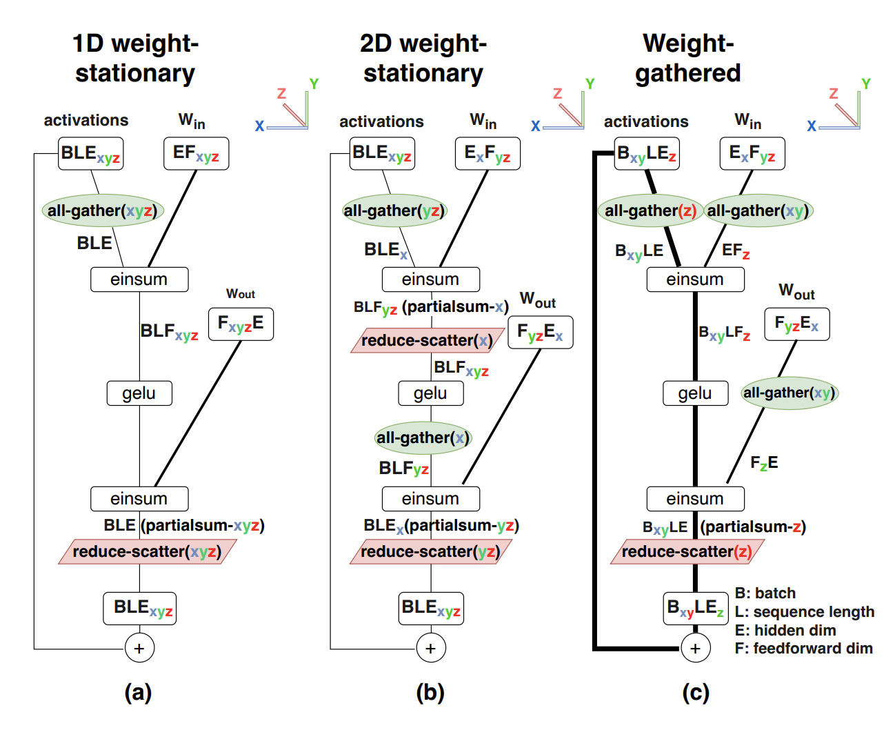
Here is a visual summary from the paper on three of the configurations described:
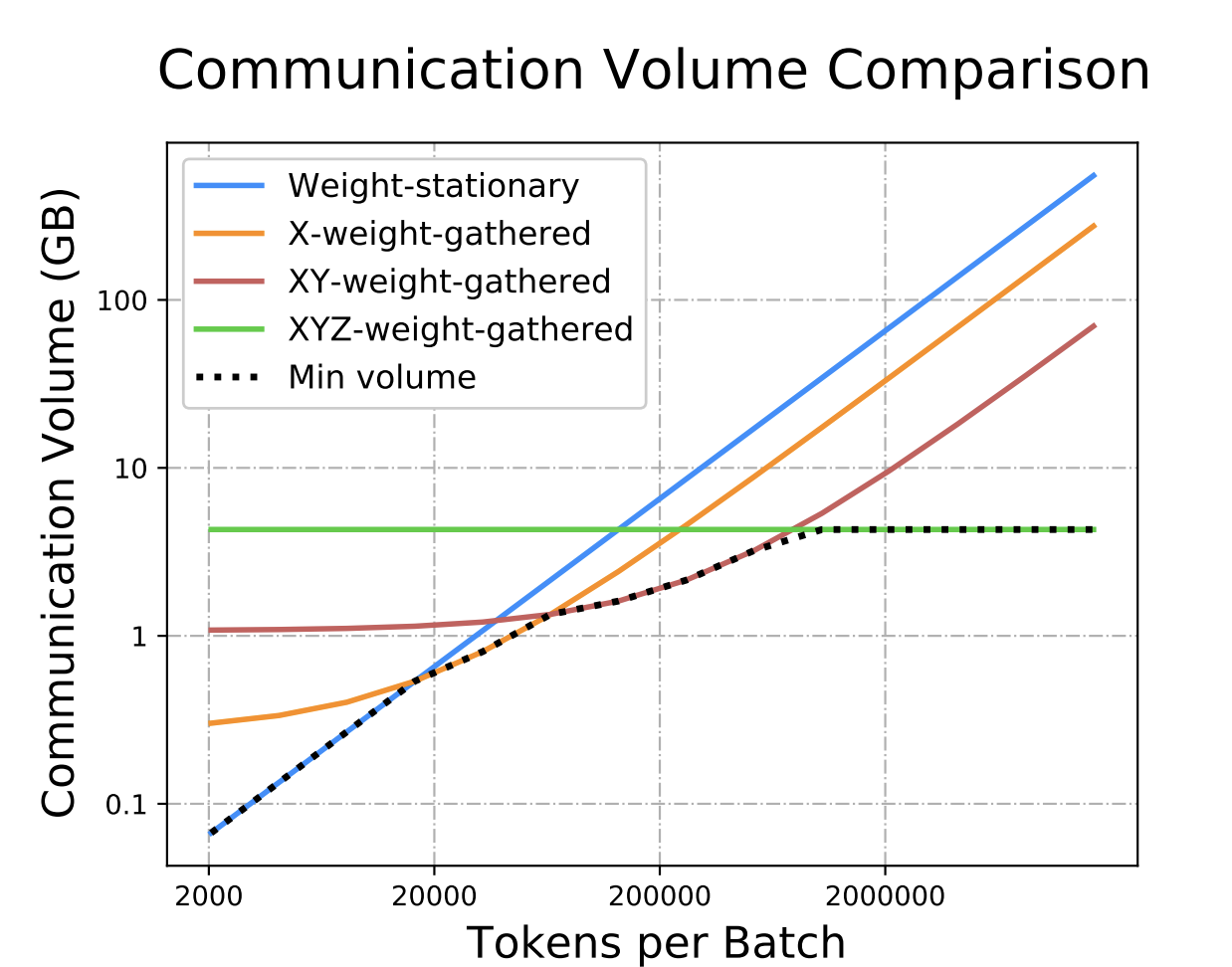
The optimal configuration, the one with the minimal communication cost for the MLP, changes as the tokens per batch increases, resulting in this elegant pareto frontier:
Partitioning The Attention Layer
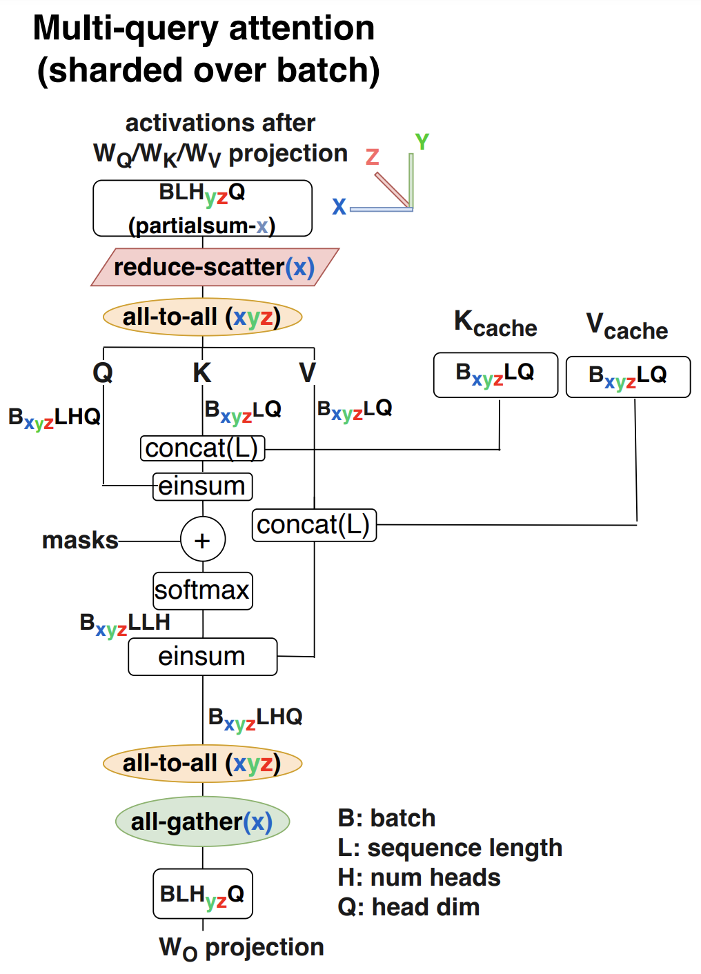
Multihead attention can be similarly parallelized due to the similar structure to the MLP (matmul, independent computations over heads, then matmul again). However, the KV cache will dominate costs with full multihead attention, most transformers these days use multiquery or grouped query attention, where there are n_heads for the query tensor, but the key and value heads are replicated. In multiquery attention, every query head shares the same key/value head, whereas grouped query attention relaxes this to produce group_size kv heads. This architectural improvement is designed to reduce the memory impact of the KV cache, as it reduces its size by a factor of n_heads / group_size where group size = 1 for multiquery attention.
Even with multiquery attention, loading the KV cache dominates memory time during decoding.Unfortunately, this performance improvement eliminates an opportunity for parallelism over the head dimension. To avoid k/v replication, we can only really shard the computation over the batch dimension. This does incur an additional all-to-all communication operation, but otherwise the $W_Q$ and $W_O$ weights behave as they do in the MLP and in the attention mechanism everything is sharded as $B_{xyz}…$ to minimize time to load the KV cache.
During prefill, however, this all-to-all communication is more expensive and there is no KV cache to load. So the attention computation is sharded over heads, and the K/V vectors are replicated for multihead attention.
Additional Optimizations
The authors further improve performance via:
- low level optimizations to improve communication and computation overlap
- int8 weight quantization (but not activation/kv cache quantization!)
- PaLM uses parallel attention and MLP layers, which allows for larger fused matmuls and “eliminates one of the all-reduces needed for $d_{ff}$/$n_{heads}$ parallelism” (n.b. I am not certain what this means exactly as the communications described do not include all-reduces, just all gathers and reduce scatters.) A non-parallel version has 14% higher inference latency, mostly due to increased communication of activations.
They reserve 30% of HBM (chip memory) for the KV cache, but do not address how it is allocated or whether it is used efficiently a la VLLM.
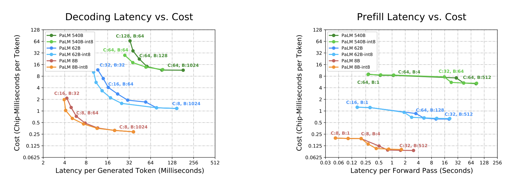
And the final results, in graph form:
And in table form:
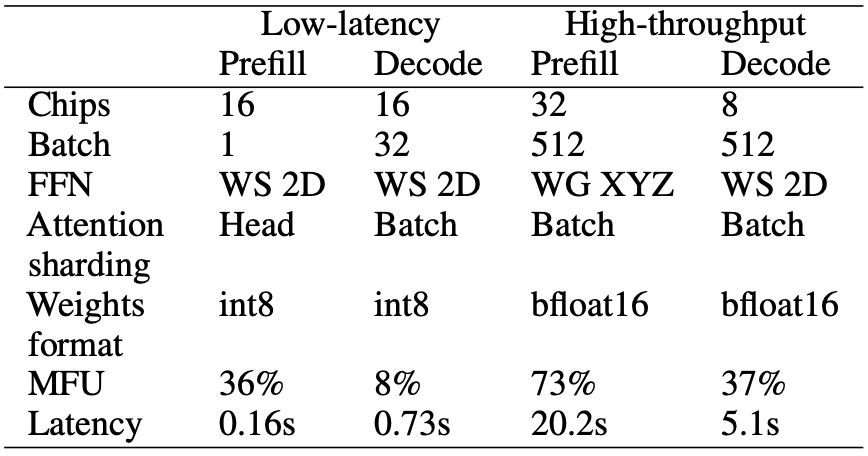
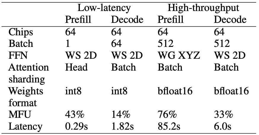
The left table shows performance numbers for the 62B model, and the right for the 540B model. Curiously, the MFU for latency sensitive batched decoding is much lower than training or throughput-oriented inference–at around 10% on TPU’s with a lot of engineering effort! Memory and communication are still the bottleneck. There is certainly performance on the table, perhaps with quantized KV cache / activations + speculative decoding tricks. Additionally, I suspect the most interesting applications will produce more than 64 tokens of output, and most of the time will be spent in the decoding phase.
At least for google, the lowest latencies are at pretty high chip counts (>8 at least). Adapting this work to a two-tier communications model and reproducing the pareto frontier with NVIDIA GPU’s would certainly be interesting, as would combining this with Pipeline Parallelism as the work is mostly orthogonal.
TL;DR
Inference is important. How does one best run large transformer for inference? Communication/memory is the bottleneck, rigorously analyze the communication + memory costs of various partitioning strategies for MLP/attention. Optimal partitioning strategy and batch/chip count changes with tokens per forward pass, prefill or decoding, and optimizing for latency or throughput. Specific results are mostly only applicable to TPU’s but one can improve on basic tensor parallelism for inference.