Speculative Decoding
Speculative Decoding
LLM inference will constitute an increasingly large proportion of compute cost. Unfortunately, for autoregressive LLMs, it is slow. Speculative decoding is a clever technique described by both Leviathan et al. 2022 and Chen et al. 2023, two concurrent papers (somewhat amusingly, from Google Research and Deepmind respectively). I’ll explain the technique, its derivation, and newer variants in this post.
Autoregressive sampling is typically memory bandwidth bound since tokens are sampled one-by-one. Each new token requires a forward pass of the entire model on the most recent token, and all model parameters to be loaded from GPU memory. This results in low utilization of compute cores when doing decoding in latency sensitive contexts. MFU (Model FLOP-s Utilization, a ratio between actual and ideal throughput on hardware) numbers are below $10\%$ during decoding after optimizations! (See Pope et al. 2023 and my notes thereof).
Algorithm
The basic premise is to produce multiple tokens per forward pass of our model. A cheap “draft” model will produce $k$ draft tokens, which may or may not be the correct continuation. Then our main expensive model will check whether the tokens are right all at once. Speedups occur when this verification is approximately as expensive as producing one token, which is true in low-batch size cases. Evaluating the likelihoods of a short sequence of $k$ tokens in parallel has a similar latency to sampling a single token. As Chen et al. more precisely describe:
- In the MLP layer, time to load the linear weights dominates compute time, so it is similar for $k$ and $1$.
- In the attention layer, the KV cache size is independent of $k$ and loading it from memory dominates memory bandwidth
- At small batch sizes and small $k$, activation communication is latency bound rather than throughput bound so the cost is similar for $k$ and $1$ tokens.
(I’ll call this The Assumption – we will look at where it breaks down later on)
We’ll assume for now that our draft model is a smaller language model. How do we actually implement the “checking” portion of the algorithm?
A naive version of speculative decoding would be to sample from the probabilities on those draft tokens one by one, and whenever the token sampled is not what the draft model produced, exit. It is easy to see that the resulting tokens are sampled from $p(x)$. However, the per token acceptance rate is $\sum_{x_i \in V} p(x_i) q(x_i)$ which for high-entropy tokens and nonzero temperature may be quite poor (e.g. for two uniform distributions over $n$ tokens our acceptance rate is $\frac{1}{n}$).
Speculative decoding works differently. We’ll call the target model distribution $p$ and the draft model distribution $q$. $p(x)$ is shorthand for $p(x_t|x_0…x_{t-1})$. Speculative decoding operates token-by-token so we don’t need to worry about interactions across token positions. The algorithm does the following in a loop:
- Produce $k$ draft tokens using the draft model $q$. Evaluate their likelihoods under $p$, which produces $k+1$ logits. For each token:
- If $p(x) > q(x)$, accept the token and continue.
- Otherwise, accept the token with probability $\frac{p(x)}{q(x)}$. If accepted, move onto the next draft token.
- On the first rejection, sample a token from the modified distribution
$p’(x) = \text{norm}(\text{max}(0, p(x)-q(x)))$ and exit. - If no tokens are rejected, sample an additional token from $p(x)$ (remember we get $k+1$ logits!)
Derivation of these distributions are in Appendix A.1. The coolest part about speculative decoding is that you can prove the resulting distribution of tokens is exactly $p$ regardless of the distribution $q$. This leads to exciting opportunities to do whatever we want to $q$ without worrying about it negatively affecting our LLM product. An n-gram model, an LLM, a process which produces deterministic tokens, could all take the place of $q$, and the resulting samples will still be from $p(x)$.
Note that $p$ and $q$ are distributions over tokens and $q$ needs to represent the probabilities of producing the draft tokens. This means that $p$ and $q$ should be measured after topk/top-p adjustments to the LLM token probabilities. There are two interesting special cases:
- Greedy decoding: $p$ is $1$ on one token and $0$ elsewhere. Of course, the algorithm accepts every $x$ which is the most likely independent of $q$
- $q$ is greedy and has probabilities $1$ on the draft tokens and $0$ elsewhere. Then we accept its tokens with probability $p(x)$. This is the case if the draft tokens are deterministic w.r.t. the preceding tokens–more on this later.
Analysis
Theoretically, how much speedup can we expect to see? Assume there is a token-wise acceptance rate (assuming independence, which isn’t true at all) $\alpha$, we can compute the expected length per step of speculative decoding $\tau$ as:
$$ \tau = \frac{1 - \alpha^{k+1}}{1 - \alpha} $$
$\tau$ is strictly greater than 1 for every $\alpha$ and approaches $k+1$ as $\alpha \rightarrow 1$. Let’s call the latency ratio between draft model latency and target model latency $c$ ($<1$). Then cost for each draft token sequence is $T_{target} \cdot c \cdot k + 1$. If we produce $\tau$ tokens on average, we can compute the ratio of the token costs to get the expected speedup:
$$ \mathbb{E(speedup)} = \frac{\tau}{kc+1} = \frac{1-a^{k+1}}{(1-\alpha)(kc+1)} $$
So a good draft model has high speedup, and so we should aim to reduce cost, and increase the acceptance rate. and fit well on the same inference hardware as the target model. The relationship between $c$ and $\alpha$ is not immediately clear, if we use a larger model we can get a better $\alpha$ at the cost of higher $c$. In practice it seems like $c \leq 0.1$ is reasonable, but we don’t quite have scaling laws to determine $\alpha$ as a function of inference latency $c$ or parameters. One can show that $\alpha$ is exactly the $1-\text{TVD}(p,q)$ where $\text{TVD}(p,q)$ is the Total Variation Distance between $p$ and $q$.
Results
How much faster is speculative decoding?
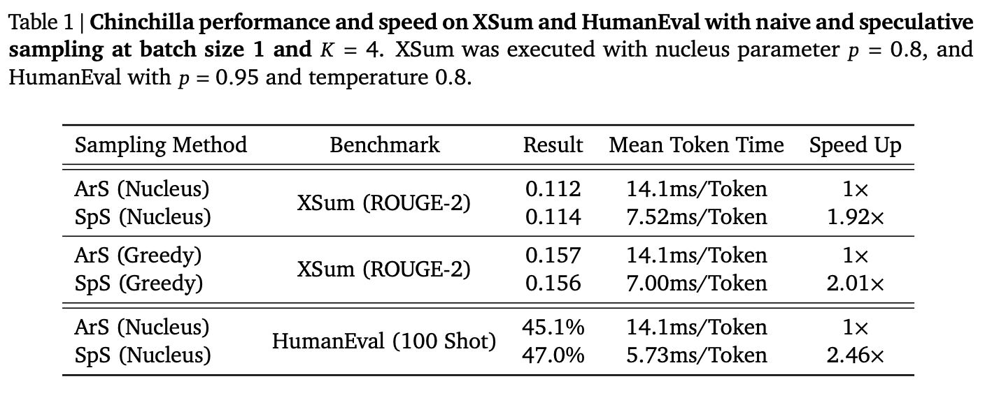
These results are from from [Chen et al. 2023], who use a 4B parameter extra-wide draft model to accelerate Chinchilla 70B. The speedup is task dependent, since the agreement rates between draft and target models will be higher on simpler, more repetitive data. Code is particularly “compressible” in this sense.
Their draft model is extra-wide because the draft model needs to run on the same hardware as the original model, and wide models are easier to split with tensor parallelism aspect ratio doesn’t narrowly matter.
Batch Size
Virtually all speculative decoding papers only discuss the single batch case, because the highest speedup comes at batch size 1. But most LLM applications other than local inference will be batched: if you are fortunate to have sufficient users you will be batching as well. Karpathy implies GPT-4 runs at batch size 256. So how does batch size influence speculative decoding?
Roughly speaking, at small batch sizes speculative decoding should still provide speedups since linear layers are memory bound for batch sizes in the tens on A100’s. If the cost ratio between running the model on one token and running on the draft tokens is $\beta$, the expected speedup is:
$$ \mathbb{E(speedup)} = \frac{1-a^{k+1}}{(1-\alpha)(kc+\beta)} $$
So the highest $\beta$ can get while offering speedups is: $$ \beta \le \frac{1-\alpha^{k+1}}{1-\alpha} - kc $$ ($k=5$, $c=.01$, $\alpha = \frac{2}{3}$ $\implies$ $\beta \lessapprox 2.69$)
The Assumption posits that $\beta \approx 1$. But at very high batch sizes, the matmuls become compute bound and $\beta$ gets closer to $k$. Speculative decoding always costs more FLOPs, so in the compute bound regime this is not good. The one place it does save time is in the attention operation, which is dominated by loading the KV cache–this cost is amortized across $\tau$ tokens.
$\beta$ is best measured for your specific setup to determine whether to apply speculative decoding. I was surprised to find that $\beta$ for batch size $2$ on gpt-fast with int8 quantization was enough to make speculative decoding not worth it. This is a result of torch.compile generating efficient code for matrix-vector multiplies at batch size one, which can be fused with dequantization. compile does not codegen at batch size 2, so the GEMM & dequant are not fused. This isn’t a universal property of inference, a fused GEMM-dequantization kernel would fix this particular case $^1$.
Mixture of Experts
The Assumption (computing likelihoods for $k$ tokens has similar latency to sampling a single token) is not true for top-k routed MoE models in the small-batch case. Let’s assume our MoE model picks two experts per token per layer (e.g. it is a top-k routed model with k=2). If you pass one token through a routed MOE layer, you will load the weights of 1 or 2 experts. But if you pass two tokens ($k=2$), combined they may pick up to 4 experts. When we are memory bandwidth bound, this is terrible because we need to pay the memory cost to load those expert weights! This doesn’t double latency exactly, but increases it substantially. So at batch size 1, speculative decoding probably won’t offer speedups for MoE models.
At moderate batch sizes, however, you typically pay for the cost to load most of the experts even with one token, so $\beta$ is only slightly $>1$. However, this is an unideal case to run MoE anyway as you are memory bound but only computing on $\frac{k}{E}$ tokens. $\beta$ is only low because your baseline inference is slow at moderate batch sizes.
Lets compute the expected number of experts loaded as a function of tokens. Let’s call the token count $T$ and the number of experts $E$. Each token uniformly (by assumption) chooses $k_\text{exp}$ of $E$ experts, and we want to count the total number of experts chosen.
- For each of the experts, we can define an indicator $X_i$ where $X_i = 1$ if expert $i$ is picked, and $0$ otherwise.
- By linearity of expectation, the expectation of the number of unique experts is the sum of the expectations of these indicator variables. So we’re interested in $$\sum_i \mathbb{E}[X_i] = \sum_i Pr(X_i) = E \cdot Pr(X_i)$$
- The probability an expert is selected by any of the tokens is $$1 - Pr(\text{Not selected}) = 1 - (\frac{E-k_{\text{exp}}}{E})^{T}$$
- So the expected number of experts is $$E\cdot(1 - (\frac{E-k_{\text{exp}}}{E})^{T})$$
Let’s do an example. Mixtral 8x7B has 8 experts per layer and top-2 routing. So for a speculate $k=5$, we have $\mathbb{E}[\text{Experts}] = 8 (1 - (\frac{2}{8})^{5}) \approx 6.101 $. For the one-token case, the expected expert count is $2$. Then the memory ratio of matmuls for MoE with 5 tokens to 1 is an estimate for $\beta$, and then $\beta \approx 3.05$ which is very large.
Note: Since speculative decoding speeds up the attention mechanism by amortizing KV cache loads over $\tau$ tokens, it’s possible that it may result in a performance improvement in the very-long-sequence high-acceptance regime despite a slowdown on the matmuls.
Draft Model Distillation
How do we get a high acceptance rate? The acceptance rate increases when our draft model more accurately matches our target model. To this end, we can use Knowledge Distillation to train the draft model efficiently to reproduce the target model’s outputs. We don’t really care if the draft model is particularly good at any downstream task, we just want it to match the target model as well as possible.
Knowledge distillation for LLM’s is not straightforward. Standard distillation procedures such as minimizing the KL divergence (KL) between the teacher and the student do not perform well at generation time.
This is because forward KL divergence $KL(P||Q)$ where $P$ is the teacher and $Q$ is the student pushes the student model to “cover” the modes of the target distribution–it will put probability wherever the target has. Since the student is weaker, it doesn’t have the capacity to also have probability wherever the teacher does.
Mode covering behavior is especially bad for sequences, because you risk sampling bad tokens, upon which errors compound during generation. The solution is to use the reverse KLD, e.g. the KL between the student and the teacher model, or a mixture of the two. See appendix A.2 for mathematical details.
Note that to optimize the reverse KL, we need to sample from the draft model rather than from the teacher model to produce sequences, and then optimize draft likelihoods to match the target model. For more details on LLM distillation in general, see the GKD paper.
The authors of DistillSpec investigate the optimal training recipe for distillation of draft LLM’s for SD and find:
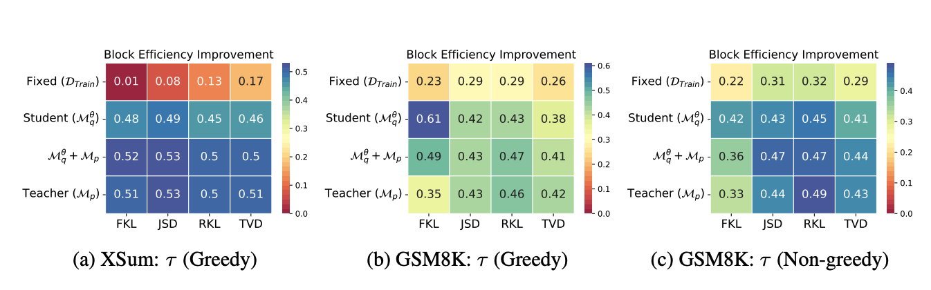
Each cell value corresponds to the relative improvement in $\tau$ (more is better), the $x$ axis lists divergences, and the $y$ axis lists from where the inputs were sampled. The main results are that
- Distilled draft models result in additional speedups.
- The best draft distillation recipe is dataset sepecific, but generally training with JSD or RKL on draft model outputs is competitive and cheap.$^2$
Interestingly, directly optimizing the TVD (Total Variation Distance, $\alpha = 1 - \text{TVD}$) does not result in the best distilled draft models.
Variants
Online Speculative Decoding
Since we are free to change our draft model as we wish to maximize the value of the speedup above, which is determined by how well the draft model approximates the target model during generation. Online Speculative Decoding leverages several insights to adapt the draft model during serving with minimal overhead to achieve higher acceptance rates and thus larger speedups.
First, optimizing the Reverse KL under the draft model distribution consists of:
a. Drawing samples from the draft model
b. Getting the probabilities from the target model on those samples
c. Computing a loss and taking an update step
(a) and (b) sure look do familiar. We already do them during speculative decoding.
Second, the draft model is so small that taking update steps on it is not that expensive.
Third, the user query distributions shift. Since the draft model is small, it behooves us (vigorous handwaving) to allocate its limited capacity to the exact distribution of user queries.
So (1) and (2) imply that continually distilling the model may be pretty cheap, and (3) implies it may be a good idea. The authors argue that we can hide all of the cost of updating the model live by doing it when there are low request volumes and it should be done on the inference hardware. Potentially true but it sounds like a massive headache (speculative decoding already is one).
Online Speculative Decoding: The Algorithm looks much like speculative decoding, but we maintain a fixed-length buffer of sequences along with the target model’s token-wise likelihoods for training later on. The authors propose doing one update step on the buffer and flushing it every $L$ sequences for some $L$. Here’s the cool chart:
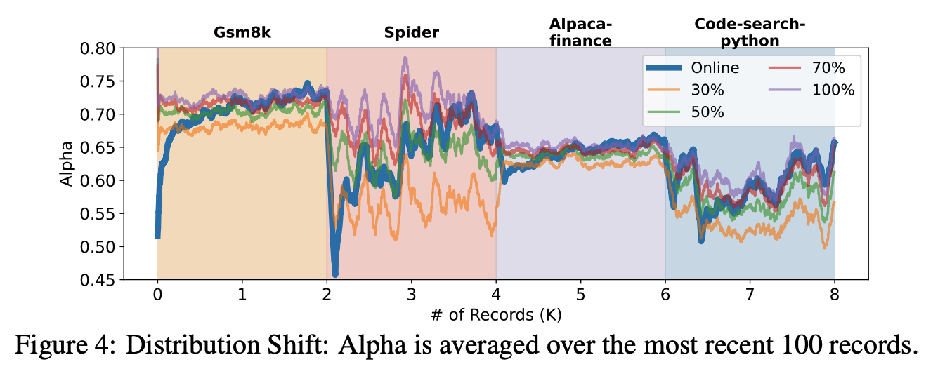
OSD is in blue, and the comparisons are draft models trained on some proportion of the specific dataset in that region. The comparision is quite unfair to OSD since we do not know the upcoming distribution ahead of time.
The authors find that one can get substantially improved acceptance rates with the distillation technique and that the draft model can adapt to new distributions reasonably well.
Correctly implementing batched speculative decoding with appropriately timed draft model distillations to your draft model on the inference hardware without OOM’s, catastrophic forgetting, or performance regressions integrated with your model runtime is left as an exercise to the reader. I suspect that saving the sequences + logits to disk, training the model on separate hardware, and redeploying draft models periodically reduces complexity.
Non-LM Draft Models
$$ \mathbb{E(speedup)} = \frac{1-a^{k+1}}{(1-\alpha)(kc + \beta)} $$
If your draft model is very cheap, $kc \approx 0$ and the expected speedup is approximately $\frac{1-a^{k+1}}{(1-\alpha)(\beta)}$. As long as $\beta \approx 1$ we can get performance improvements. The most simplest zero cost draft models are N-gram models. Another option is to use n-grams, but only if they exist in your prompt–this gives Prompt Lookup Decoding. If the n-gram does not exist in your prompt, fall back to standard decoding.
The reason these work is that without speculation, LLM’s need to produce very obvious sequences of tokens despite not needing that much compute to do so, leading to a nontrivial acceptance rate. For problems with repetitive subsequences (code, especially if long context w/RAG), some fusion of zero cost and standard draft modeling makes the most sense. How exactly to fuse them is probably an interesting avenue to investigate, as when you have long trivial / copied sequences you should try to “sample” from prompt lookup type methods but otherwise fall back to a draft LLM.
Another use for zero-cost draft models is to accelerate a non-zero cost draft model. The draft model itself suffers from sequential decoding problems and is also probably memory bandiwdth bound, even if it is smaller! Staged Speculative Decoding proposes to accelerate a small LLM draft model with an N-gram model, leading to this aesthetic visualization:
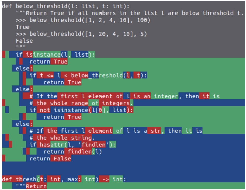
Green tokens are accepted N-gram tokens, blue tokens are generated by the draft (40M model) and red tokens are generated by the base model (GPT-2). Unfortunately GPT-2 does not do too well at coding. It would be interesting to take a look at this with a more capable series of models.
Not technically speculative
Medusa attaches additional heads at the end of a pretrained model to predict $p(x_{t+2}|x_{1…t})$, $p(x_{t+3}|x_{1…t})$ etc. They use this to generate a tree of draft tokens which are evaluated in parallel. Medusa does not exactly match the distribution in non-greedy settings (they use an approximate “typical acceptance” scheme), which makes me somewhat suspicious, but it seems reasonable for greedy generation and you don’t need access to a pretrained small model on the same tokenizer.
TL;DR
Speculative decoding speeds up memory-bound decoding of dense transformers which is mostly orthogonal to other inference acceleration methods. If a suitable draft model is available (or n-grams are good enough) and the complexity of implementation is moderate, speculative decoding offers substantial performance improvements. Draft models should be distilled from the target model either offline or online, this pays for itself. However, speculative decoding is not useful for compute-bound inference with large batch sizes.
Acknowledgements and Footnotes
$^1$ Thanks to Horace He who answered some of my questions about this. His blog and twitter are truly excellent resources for ML systems performance info.
$^2$ The OSD paper actually finds that training forward KL under the teacher distribution led to the highest acceptance rate–I think the experiments in DistilSpec are the most thorough. Unfortunately there isn’t yet a single winning configuration across all datasets.
Appendix
A.1 Deriving SD Equations
One can prove that for a particular token, the likelihood of it being sampled is the same as $p(x)$. I was personally interested in how these equations are derived. Imagine two partially overlapping probability distributions:
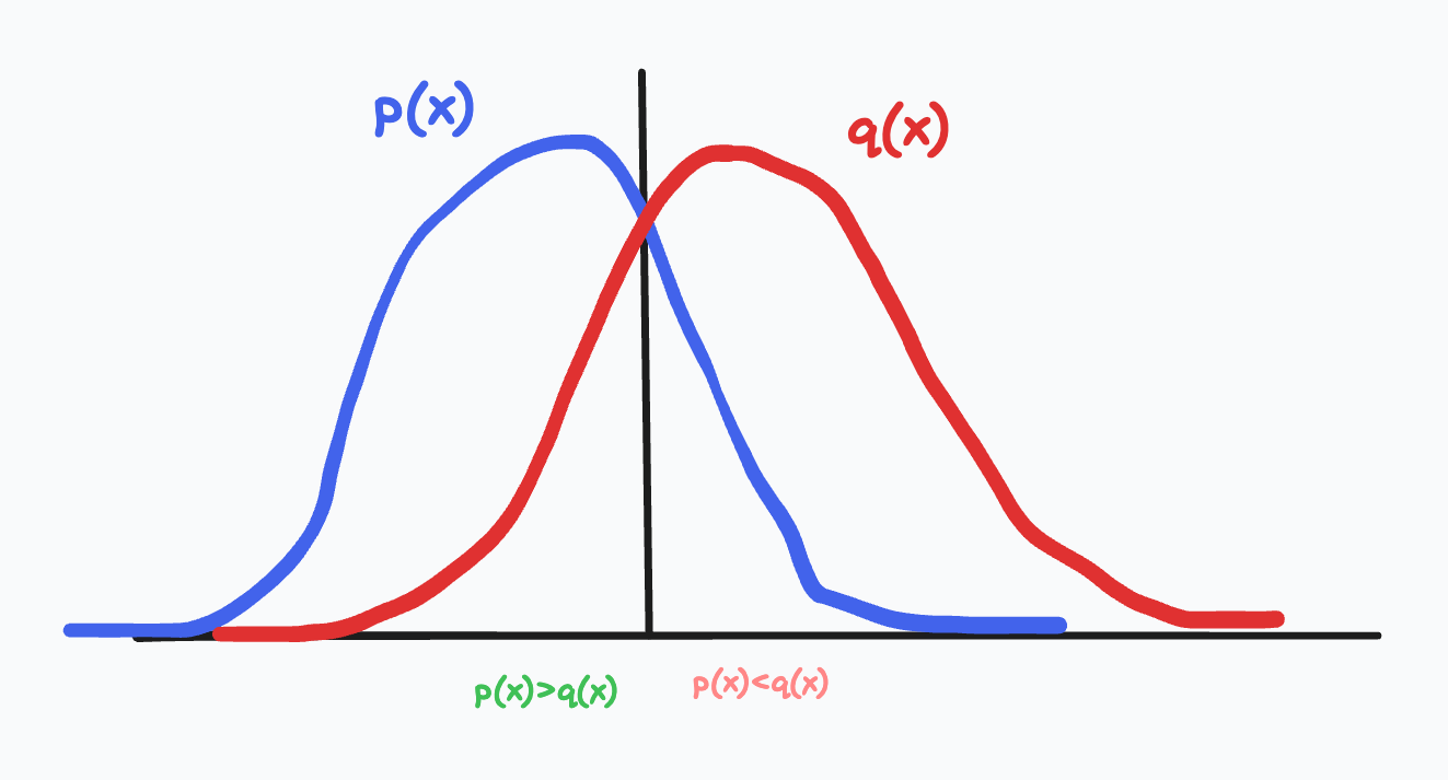
The goal in this toy scenario is to produce samples from $p$ with a sample from $q$. If the acceptance likelihood is their overlap, we need the rejection case to move the likelihood in the rightmost part of the graph ($q > p$) to the leftmost part of the graph $p > q$.
The draft model produces points $x \sim q$, and the probability of drawing that point is $q(x)$. There are two cases:
- $p(x) < q(x)$
- $p(x) \geq q(x)$
For the first case, $p(x) < q(x)$, we will accept it with probability $\frac{p(x)}{q(x)}$. As long as there is no other way to generate $x$ from our process, we know that the probability of getting x is $q(x) \frac{p(x)}{q(x)} = p(x)$. If we reject it, we will sample it from some other distribution $p’(x)$, which we will work out shortly.
For the second case, $p(x) \geq q(x)$, we will always accept it. But we still have to make up $p(x)-q(x)$ probability. This is where the rejection cases from (1) come in. For any $x$ where $p(x) \geq q(x)$, the rejection distribution $p’(x)$ needs to result in $p(x) - q(x)$ additional probability at $x$. More precisely, $\int_x P(\text{reject}) * p’(x) = \text{max}(p(x) - q(x),0)$ where the $\text{max}$ comes from the fact that we are only interested in areas where $p(x) >= q(x)$, and we cannot produce $x \text{ s.t. } p(x) < q(x)$ from case (1) after rejection.
However, we don’t need to analytically compute $\int_x P(\text{reject})$ since it’s a constant w.r.t. $x$ therefore
$$p’(x) = \text{norm}(\text{max}(p(x)-q(x),0))$$
In the speculative decoding case, we apply this sampling scheme at each token and stop on the first rejection. We need to stop on the first rejection because the sampled token will not be the draft token, so the subsequent $q(x_{t+1})$ will be incorrect as they condition on a different $x_t$.
A.2 KLD and mode-covering
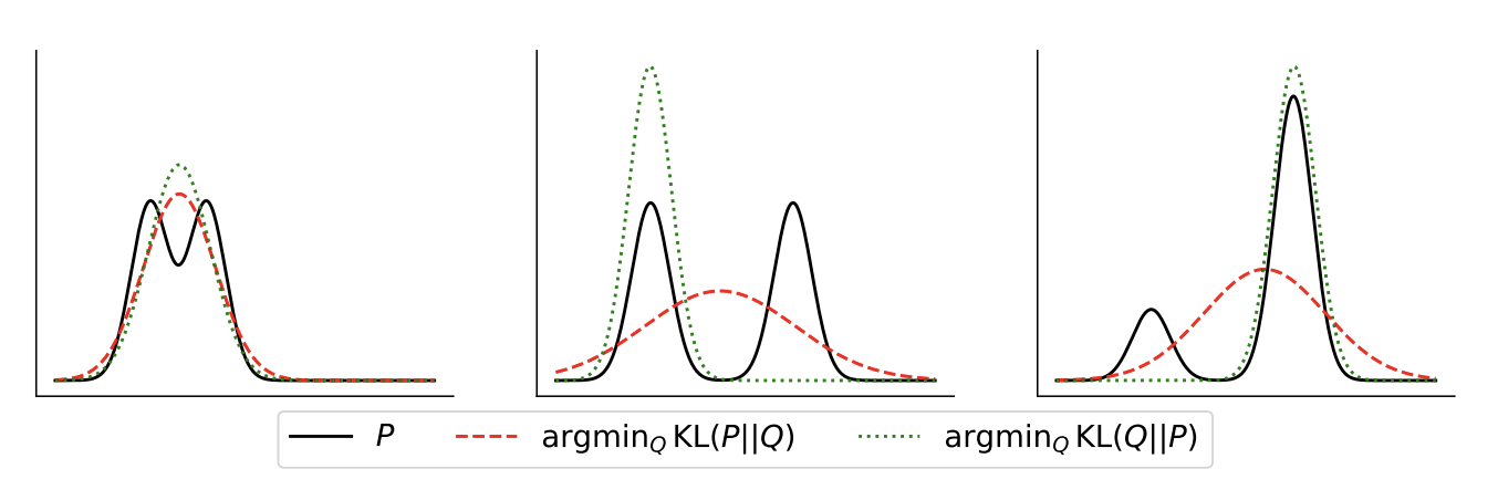
The above figure, taken from Agarwal et al. 2023, shows the different behaviors of optimizing a gaussian $Q$ to minimize either the KL divergence or the reverse KL divergence with $P$.
The argmin of the forward KL places mass wherever $P$ places mass, but the argmin of the reverse KL places no mass where $P$ has no mass. Forward KL optimization causes mode covering, but reverse KL optimization causes mode seeking.
Why? Recall that the KL divergence between distributions $P$ and $Q$ is:
$D_{\text{KL}}(P || Q) = \mathbb{E}_{x \sim p} \log \left( \frac{p(x)}{q(x)} \right) $
It is not symmetric between $P$ and $Q$. For our purposes, this forward KL divergence is between the target $P$ and the draft $Q$. If $q(x)$ is very small for some sequence drawn from $p$ this loss gets very large and is unbounded. So $q$ will “attempt” to put at least some probability wherever $p$ has probability, and if $q$ is weak it will result in mode seeking behavior.
This is undesirable for sequences because samples from $q$ will “veer off course” since we will pick tokens which are very unlikely under $p$ and then compound on that error by sampling tokens given the unlikely ones.
$D_{\text{KL}}(Q || P) = \mathbb{E}_{x \sim q} \left[ \log \left( \frac{q(x)}{p(x)} \right) \right]$
On the other hand, if the draft/student is mode-covering, we will sample low-diversity sequences.
As an aside, the standard langauge modeling objective is the same as minimizing the KL between $P$, the empirical distribution of language in the dataset, and your model $Q$. So we should expect diverse, mode covering behavior with mass where the underlying distribution has none, especially with smaller models. But, RLHF does not optimize a similar KLD–so perhaps this is part of the explanation as to “why” RLHF reduces diversity?